Part I built one camera, and Part II established the constraint between two images:
\[ x'^{\mathsf T}Fx=0. \]Part III asks the computational question left open by that equation: given noisy point matches, how do we actually estimate (F)? The answer begins as linear algebra, but it ends as an estimation problem. The bridge is the normalized 8-point algorithm.
From many tentative matches, estimate one matrix that makes their epipolar geometry mutually consistent.
The Input Is Correspondence, Not 3D Reconstruction
Assume a matcher has supplied image correspondences
\[ x_i\leftrightarrow x'_i, \qquad x_i=(x_i,y_i,1)^{\mathsf T}, \quad x'_i=(x'_i,y'_i,1)^{\mathsf T}. \]The coordinates are homogeneous image points. At this stage we do not know the 3D point that generated either observation; we only hypothesize that both points depict the same scene location. If the hypothesis is correct, the pair must obey
\[ x_i'^{\mathsf T}Fx_i=0. \]So the objective is not to fit a line to points in one image. It is to find one 3 × 3 matrix F that makes every first-image point induce an epipolar line in the second image on which its partner lies.
Why the Fundamental Matrix Has Seven Degrees of Freedom
The 3 × 3 matrix F has nine entries, but its homogeneous scale carries no geometry:
\[ F\sim\lambda F, \qquad \lambda\ne0. \]That removes one degree of freedom. A valid fundamental matrix must also be singular,
\[ \det(F)=0, \qquad \operatorname{rank}(F)=2, \]which removes one more. Thus the set of valid fundamental matrices has (9-1-1=7) degrees of freedom. This explains two names that otherwise sound contradictory: seven correspondences are theoretically minimal, while eight correspondences give a particularly convenient linear algorithm.
One Match Becomes One Row of a Linear System
Write the entries of (F) as one vector,
\[ f=(f_{11},f_{12},f_{13},f_{21},f_{22},f_{23},f_{31},f_{32},f_{33})^{\mathsf T}. \]Expanding the epipolar constraint for one correspondence produces
\[ \begin{bmatrix} x'x & x'y & x' & y'x & y'y & y' & x & y & 1 \end{bmatrix}f=0. \]Every point pair contributes one such row. Stacking (n) pairs gives
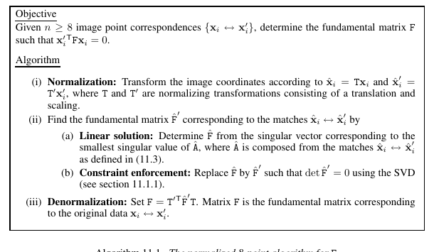
\[ Af=0, \qquad A\in\mathbb R^{n\times9}. \]With eight or more non-degenerate matches, the direct estimate is the unit vector f in the right null-space of A. With noisy data, this becomes a least-squares problem. This is where the first SVD appears:
\[ A=U_A\operatorname{diag}(s_1,\ldots,s_9)V_A^{\mathsf T}, \qquad s_1\ge\cdots\ge s_9. \]The last column of VA is the right singular vector associated with the smallest singular value s9. It is the unit vector that makes Af as small as possible, so we take it as f and reshape its nine entries into a 3 × 3 matrix F̂.
This is the entire linear heart of the 8-point algorithm. The fact that it is linear is useful, but it also hides two issues: the raw solution usually has rank three, and pixel coordinates make the system poorly conditioned.
Rank Two Is a Geometric Requirement
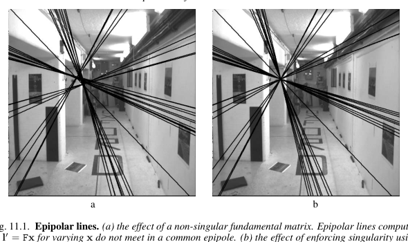
The unconstrained least-squares matrix F̂ is merely close to a fundamental matrix. Noise means it will generally have three non-zero singular values. But a real F has a left and a right null vector—the epipoles—so it must have rank two.
This calls for a second, separate SVD. It is not used to solve the point equations; it repairs the geometry of the matrix obtained from the first SVD. Take
\[ \hat F=U_F\operatorname{diag}(\sigma_1,\sigma_2,\sigma_3)V_F^{\mathsf T}, \qquad \sigma_1\ge\sigma_2\ge\sigma_3. \]Set the smallest singular value to zero and reassemble:
\[ F=U_F\operatorname{diag}(\sigma_1,\sigma_2,0)V_F^{\mathsf T}. \]This is the nearest rank-two matrix to F̂ in Frobenius norm. In short: the SVD of A selects the best linear fit; the SVD of F̂ removes the one singular-value direction that violates epipolar geometry. The first works in a 9-dimensional vector space of matrix entries; the second projects the resulting 3 × 3 matrix back onto the geometrically legal set.
Normalization Makes the Linear Solve Trustworthy
Raw pixel coordinates may be in the hundreds or thousands while the final homogeneous coordinate is (1). Those unequal scales make (A) ill-conditioned: a small perturbation in one coordinate can produce a disproportionately large perturbation in the null-space estimate.
Hartley’s normalized 8-point algorithm first finds a similarity transform (T) for the first image and (T’) for the second such that the transformed points
\[ \tilde x_i=Tx_i, \qquad \tilde x'_i=T'x'_i \]have centroid at the origin and root-mean-square distance √2 from it. Estimate the normalized fundamental matrix from these normalized coordinates, enforce its rank-two constraint, then undo the coordinate changes:
\[ F=T'^{\mathsf T}\tilde F T. \]The transpose on T′ is not a cosmetic detail. A line transforms contravariantly: transforming an image point by T′ requires the corresponding dual transformation on a line. Thus, in original coordinates, the recovered matrix is exactly the display equation above. This is why normalization can be performed before estimation without changing the geometric relation being sought.
Seven Points Are Minimal; Eight Points Are Usually the First Tool
With exactly seven correspondences, (A) normally has a two-dimensional null-space. Let its basis matrices be (F_1) and (F_2). Every linear solution has the form
\[ F(\alpha)=\alpha F_1+(1-\alpha)F_2. \]Enforcing singularity gives
\[ \det(F(\alpha))=0, \]a cubic polynomial in (alpha). It can yield one or three real fundamental matrices. The 7-point algorithm is therefore minimal and useful inside robust sampling methods, but it has multiple candidate solutions. The 8-point algorithm uses one extra match to obtain a one-dimensional null-space and one direct linear candidate before rank enforcement.
Estimation Needs an Error Model
With real matches, no (F) makes every residual exactly zero. The scalar
\[ r_i=x_i'^{\mathsf T}Fx_i \]is the algebraic residual. It is convenient because it is what makes (Af=0) linear, but it is not a distance measured in pixels. A more geometric quantity measures the distance from a point to its predicted epipolar line; the Sampson error is a first-order approximation to that geometric reprojection error:
\[ d_{\mathrm{Sampson}}^2(x,x',F)= \frac{(x'^{\mathsf T}Fx)^2} {(Fx)_1^2+(Fx)_2^2+(F^{\mathsf T}x')_1^2+(F^{\mathsf T}x')_2^2}. \]The denominator converts the residual into an image-space scale using the line coefficients. The practical lesson is simple: linear algebra gives an initial estimate; meaningful geometry decides how to refine and evaluate it.
From the Chapter to a Real Pipeline
Feature matching produces many false correspondences, so no least-squares method should be trusted on all matches at once. A typical workflow is:
- detect and match features;
- repeatedly sample a small set of matches and estimate (F) with a normalized 8-point method, or a 7-point minimal solver;
- score every match using an epipolar distance or Sampson error;
- keep the largest consensus set with RANSAC;
- re-estimate (F) from those inliers and enforce rank two.
Chapter 9 said that (F) turns a two-dimensional correspondence search into a one-dimensional search. Chapter 11 explains how to obtain the matrix that supplies those lines from imperfect evidence.
The Five Things to Keep
- Every correspondence supplies one linear equation in the entries of (F).
- (F) has seven degrees of freedom: scale is irrelevant and rank two is required.
- The first SVD, on A, solves the noisy linear system by selecting its smallest right singular vector.
- The second SVD, on the reshaped estimate F̂, sets its smallest singular value to zero and enforces rank two.
- Both SVD steps and point normalization are essential parts of the algorithm, not optional cleanup.
- In practice, (F) is estimated robustly from noisy matches with RANSAC and a geometric error measure.
Reference
R. Hartley and A. Zisserman. Multiple View Geometry in Computer Vision, 2nd ed., Cambridge University Press, 2004. Chapter 11, “Computation of the Fundamental Matrix (F).”
Comments